|
|
|
Examples In the following three simple examples are described, which illustrate the application of our process mining approach. For each of the two first examples a log file (containing 5,000 traces) is provided below, that can be used with the ProM framework — notice that in both cases an additional task (named X) as been introduced in order to have a unique final task, as required by ProM
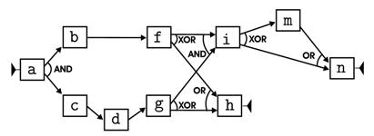
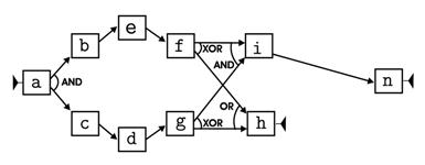
The log used in the last example is instead already provided along with ProM. If you glad, you can then experencing the usage of the DWS Mining plugin described in the section Tools on these example scenarios. Example 1A a first example, let us consider the process of handling customers’ orders within a business company, for which the following figure shows a possible workflow schema.
Figure 1 The process consists of the following activities:
We randomly generated a log containing 5,000 traces, that are all compliant with the workflow schema in Figure 1. In addition, in the generation of the log, we also required that task m could not occur in
any execution trace containing e, and
that task l could not appear in any trace containing d. By the
way, these constraints assure that a fidelity discount is never applied to a new customer and that,
respectively, a fast
dispatching
procedure cannot be performed whenever some external supplies were asked for. Let us now apply the DWS mining tool using the following values for its parameters:
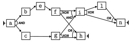
As a result we obtain a tree with a root and four leaves. The schema associated with the root is just the schema in Figure 1. However, it is only a first attempt to model the whole log with a single schema. Indeed, since it does not capture the constraints discussed above, it is not a accurate enough model for the log. The schemata of the leaves are instead reported in the following figure.
Figure 2 Each of the schemata in Figure 2 models a different usage scenarios of the process, and has been discovered by applying a classical process mining algorithm to a properly discovered cluster of traces. As a whole they constitute a disjunctive workflow schema that exactly model the log, and provides for a clearer view over the latent behavior of the process.
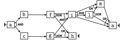
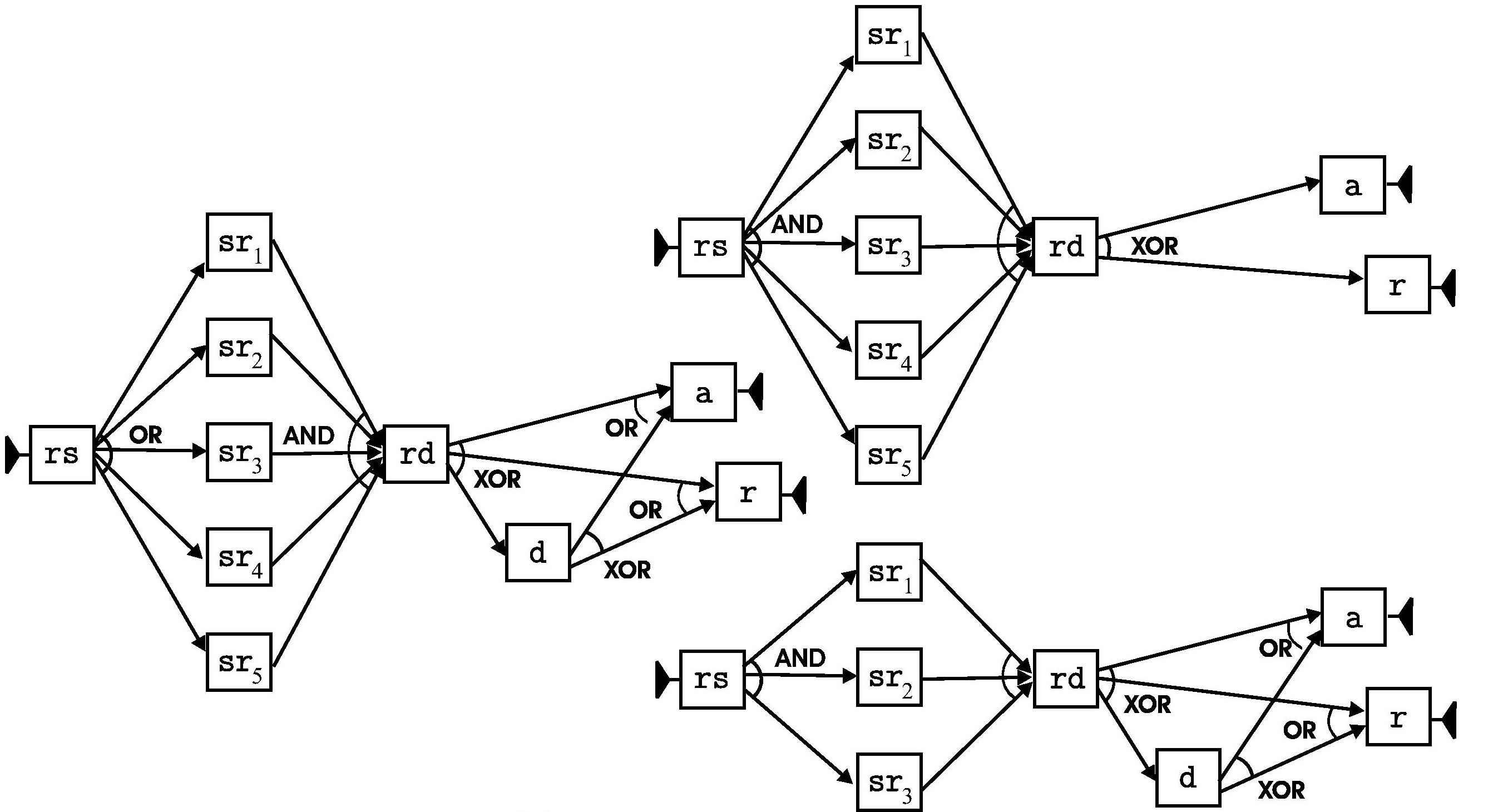
Example 2As a further example, let us consider the process of reviewing a paper submitted to a scientific conference. The process consists of the following tasks:
Actually, in the case where the paper is authored by a program committee member, it has to be reviewed by 5 reviewers and it is immediately rejected in the case some reviewer does not want it to be accepted for publication. Otherwise, only 3 reviewers are assigned to the paper.
Figure 3 A possible workflow schema for the process is reported on the left of
Figure 3 — notice According to this schema and to the above specified rules, we generated a log of 5,000 traces using a random generator. We then applied the DWS mining tool using the same values as in the previous example for all parameters, except for the nr. of clusters per split, that we set to 2. The two resulting schemas are shown on the right of the same figure. It is clear that one schema models the process for papers written by a program committee member, while the other models any other case — notice that for both schemas, rs is an and-join task, now.
Example 3The examples above show that the approach is very effective in providing insights into a process whose enactment is constrained by some kind of rules, possibly involving information that is beyond the pure execution of activities (e.g., stored in some database. This is quite a common situation in practical applications. However, even in the case where no behavioral rules are
defined and,
hence, where there is only one usage scenario, the approach is
still
useful in order to identify some (hidden) variants, which correspond to
anomalies and
malfunctioning in the system. In such a case, it is possible to recognize the
“normal” behavior of the process, along with the main groups of instances that deviate
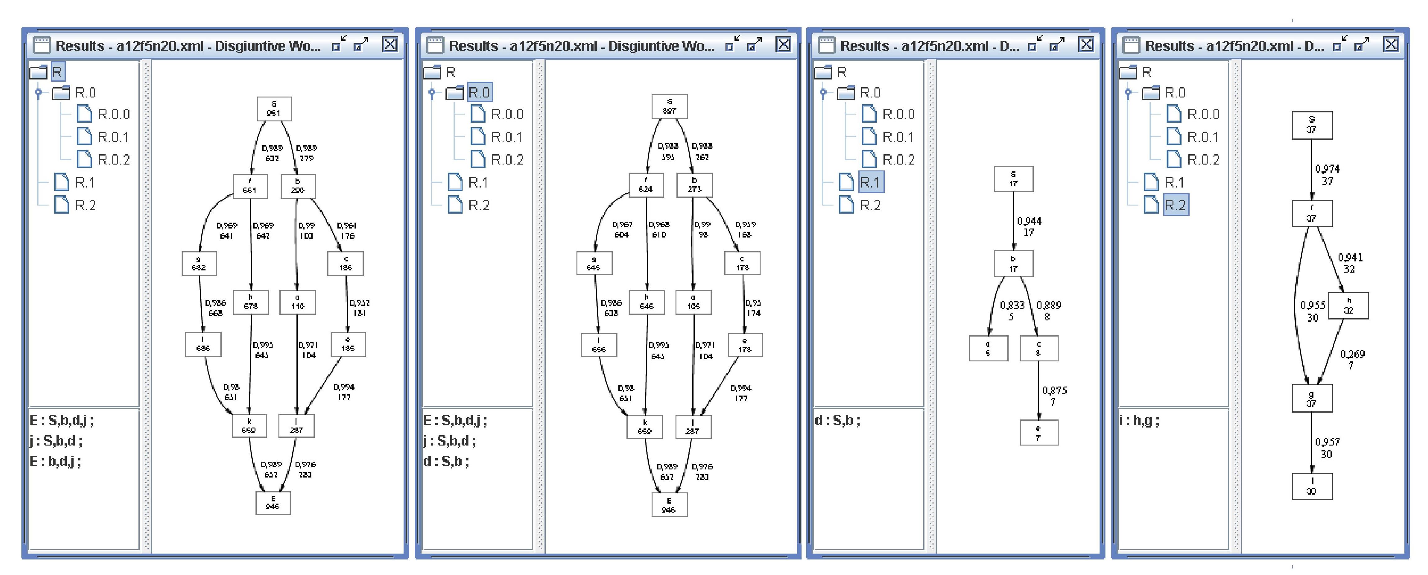
from it. As an example, we examine the results obtained with the log file a12f5n20.xml (a real data set available at http://www.processmining.org), when setting sigma = 0.01, gamma = 0.4, feature# = 3, cluster#= 3, and featureLength = 5. Figure 4 shows the hierarchy and the models associated with each node in the second level of it: one large cluster R0 is discovered whose schema coincides with that of R and then represents the typical behavior. Conversely, both clusters R1 and R2 (containing 17 and 37 traces, respectively) may be perceived as outliers w.r.t. the discovered main behavior.
|
|
|